Explainers
Simple example
In order to start an ExplainerDashboard you first need to construct an
Explainer instance. They come in two flavours and at its most basic they
only need a model, and a test set X and y:
from explainerdashboard import ClassifierExplainer, RegressionExplainer

explainer = ClassifierExplainer(model, X_test, y_test)
explainer = RegressionExplainer(model, X_test, y_test)
This is enough to launch an ExplainerDashboard:
from explainerdashboard import ExplainerDashboard
ExplainerDashboard(explainer).run()
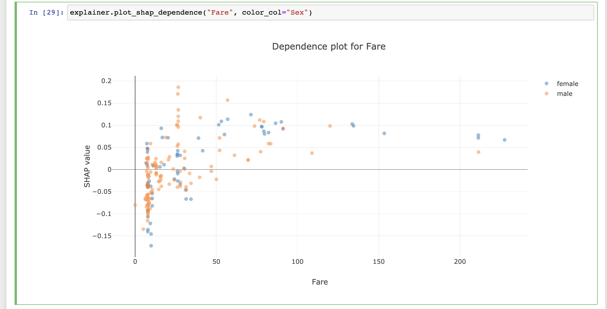
Or you can use it interactively in a notebook to inspect your model using the built-in plotting methods, e.g.:
explainer.plot_confusion_matrix()
explainer.plot_contributions(index=0)
explainer.plot_dependence("Fare", color_col="Sex")
For the full lists of plots available see Plots.
Or you can start an interactive ExplainerComponent in your notebook using InlineExplainer, e.g.:
from explainerdashboard import InlineExplainer

InlineExplainer(explainer).tab.importances()
InlineExplainer(explainer).classifier.roc_auc()
InlineExplainer(explainer).regression.residuals_vs_col()
InlineExplainer(explainer).shap.overview()
Parameters
There are a number of optional parameters that can either make sure that SHAP values get calculated in the appropriate way, or that make the explainer give a bit nicer and more convenient output:
ClassifierExplainer(model, X_test, y_test,
        shap='linear', # manually set shap type, overrides default 'guess'
        X_background=X_train, # set background dataset for shap calculations
        model_output='logodds', # set model_output to logodds (vs probability)
        cats=['Sex', 'Deck', 'Embarked'], # makes it easy to group onehotencoded vars
        idxs=test_names, # index with str identifier
        index_name="Passenger", # description of index
        descriptions=feature_descriptions, # show long feature descriptions in hovers
        target='Survival', # the name of the target variable (y)
        precision='float32', # save memory by setting lower precision. Default is 'float64'
        labels=['Not survived', 'Survived']) # show target labels instead of ['0', '1']
cats
If you have onehot-encoded your categorical variables, they will show up as a lot of independent features. This clutters your feature space, and often makes it hard to interpret the effect of the underlying categorical feature.
You can pass a dict to the parameter cats specifying which are the
onehotencoded columns, and what the grouped feature name should be:
ClassifierExplainer(model, X, y, cats={'Gender': ['Sex_male', 'Sex_female']})
However if you encoded your feature with pd.get_dummies(df, prefix=['Name']),
then the resulting onehot encoded columns should be named
‘Name_John’, ‘Name_Mary’, Name_Bob’, etc. (or in general
CategoricalFeature_Category), then you can simply pass a list of the prefixes
to cats:
ClassifierExplainer(model, X, y, cats=['Sex', 'Deck', 'Embarked'])
And you can also combine the two methods:
ClassifierExplainer(model, X, y,
    cats=[{'Gender': ['Sex_male', 'Sex_female']}, 'Deck', 'Embarked'])
You can now use these categorical features directly as input for plotting methods, e.g.
explainer.plot_dependence("Deck"), which will now generate violin plots
instead of the default scatter plots.
cats_notencoded
When you have onehotencoded a categorical feature, you may have dropped some columns
during feature selection. Or there are new categories in the test set that were not encoded
as columns in the training set. In that cases all columns in your onehot encoding may be equal
to 0 for some rows. By default the value assigned to the aggregated feature for such cases is 'NOT_ENCODED',
but this can be overriden with the cats_notencoded parameter:
ClassifierExplainer(model, X, y,
    cats=[{'Gender': ['Sex_male', 'Sex_female']}, 'Deck', 'Embarked'],
    cats_notencoded={'Gender': 'Gender Other', 'Deck': 'Unknown Deck', 'Embarked':'Stowaway'})
idxs
You may have specific identifiers (names, customer id’s, etc) for each row in
your dataset. By default X.index will get used
to identify individual rows/records in the dashboard. And you can index using both the
numerical index, e.g. explainer.get_contrib_df(0) for the first row, or using the
identifier, e.g. explainer.get_contrib_df("Braund, Mr. Owen Harris").
You can override using X.index by passing a list/array/Series idxs
to the explainer:
from explainerdashboard.datasets import titanic_names

test_names = titanic_names(test_only=True)
ClassifierExplainer(model, X_test, y_test, idxs=test_names)
index_name
By default X.index.name or idxs.name is used as the description of the index,
but you can also pass it explicitly, e.g.: index_name="Passenger".
descriptions
descriptions can be passed as a dictionary of descriptions for each feature.
In order to be explanatory, you often have to explain the meaning of the features
themselves (especially if the naming is not obvious).
Passing the dict along to descriptions will show hover-over tooltips for the
various features in the dashboard. If you grouped onehotencoded features with
the cats parameter, you can also give descriptions of these groups, e.g:
ClassifierExplainer(model, X, y,
    cats=[{'Gender': ['Sex_male', 'Sex_female']}, 'Deck', 'Embarked'],
    descriptions={
        'Gender': 'Gender of the passenger',
        'Fare': 'The price of the ticket paid for by the passenger',
        'Deck': 'The deck of the cabin of the passenger',
        'Age': 'Age of the passenger in year'
    })
target
Name of the target variable. By default the name of the y (y.name) is used
if y is a pd.Series, else it defaults to 'target', bu this can be overriden:
ClassifierExplainer(model, X, y, target="Survival")
labels
For ClassifierExplainer only: The outcome variables for a classification y are assumed to
be encoded 0, 1 (, 2, 3, ...) You can assign string labels by passing e.g.
labels=['Not survived', 'Survived']:
ClassifierExplainer(model, X, y, labels=['Not survived', 'Survived'])
units
For RegressionExplainer only: the units of the y variable. E.g. if the model is predicting
house prices in dollars you can set units='$'. If it is predicting maintenance
time you can set units='hours', etc. This will then be displayed along
the axis of various plots:
RegressionExplainer(model, X, y, units="$")
X_background
Some models like sklearn LogisticRegression (as well as certain gradient boosting
algorithms such as xgboost in probability space) need a background dataset to calculate shap values.
These can be passed as X_background. If you don’t pass an X_background, Explainer
uses X instead but gives off a warning. (You want to limit the size of X_background
in order to keep the SHAP calculations from getting too slow. Usually a representative
background dataset of a couple of hunderd rows should be enough to get decent shap values.)
model_output
By default model_output for classifiers is set to "probability", as this
is more intuitively explainable to non data scientist stakeholders.
However certain models (e.g. XGBClassifier, LGBMCLassifier, CatBoostClassifier),
need a background dataset X_background to calculate SHAP values in probability
space, and are not able to calculate shap interaction values in probability space at all.
Therefore you can also pass model_output=’logodds’, in which case shap values
get calculated faster and interaction effects can be studied. Now you just need
to explain to your stakeholders what logodds are :)
shap
By default shap='guess', which means that the Explainer will try to guess
based on the model what kind of shap explainer it needs: e.g.
shap.TreeExplainer(...), shap.LinearExplainer(...), etc.
In case the guess fails or you’d like to override it, you can set it manually:
e.g. shap='tree' for shap.TreeExplainer, shap='linear' for shap.LinearExplainer,
shap='kernel' for shap.KernelExplainer, shap='deep' for shap.DeepExplainer, etc.
model_output, X_background example
An example of using setting X_background and model_output with a
LogisticRegression:
from sklearn.linear_model import LogisticRegression

model = LogisticRegression()
model.fit(X_train, y_train)

explainer = ClassifierExplainer(model, X_test, y_test,
                                    shap='linear',
                                    X_background=X_train,
                                    model_output='logodds')
ExplainerDashboard(explainer).run()
cv
Normally metrics and permutation importances get calculated over a single fold
(assuming the data X is the test set). However if you pass the training set
to the explainer, you may wish to cross-validate calculate the permutation
importances and metrics. In that case pass the number of folds to cv.
Note that custom metrics do not work with cross validation for now.
na_fill
If you fill missing values with some extreme value such as -999 (typical for
tree based methods), these can mess with the horizontal axis of your plots.
In order to filter these out, you need to tell the explainer what the extreme value
is that you used to fill. Defaults to -999.
precision
You can set the precision of the calculated shap values, predictions, etc, in
order to save on memory usage. Default is 'float64', but 'float32' is probably
fine, maybe even 'float16' for your application.
Pre-calculated shap values
Perhaps you already have calculated the shap values somewhere, or you can calculate them off on a giant cluster somewhere, or your model supports GPU generated shap values.
You can simply add these pre-calculated shap values to the explainer with
explainer.set_shap_values() and explainer.set_shap_interaction_values() methods.
Plots
Classifier Plots
ClassifierExplainer defines a number of additional plotting methods:
plot_precision(bin_size=None, quantiles=None, cutoff=None, multiclass=False, pos_label=None)
plot_cumulative_precision(pos_label=None)
plot_classification(cutoff=0.5, percentage=True, pos_label=None)
plot_confusion_matrix(cutoff=0.5, normalized=False, binary=False, pos_label=None)
plot_lift_curve(cutoff=None, percentage=False, round=2, pos_label=None)
plot_roc_auc(cutoff=0.5, pos_label=None)
plot_pr_auc(cutoff=0.5, pos_label=None)
example code:
explainer = ClassifierExplainer(model, X, y, labels=['Not Survived', 'Survived'])
explainer.plot_confusion_matrix(cutoff=0.6)
explainer.plot_precision(quantiles=10, cutoff=0.6, multiclass=True)
explainer.plot_lift_curve(percentage=True)
explainer.plot_roc_auc(cutoff=0.7)
explainer.plot_pr_auc(cutoff=0.3)
More examples in the notebook on the github repo.
plot_precision
- ClassifierExplainer.plot_precision(bin_size=None, quantiles=None, cutoff=None, multiclass=False, pos_label=None)
plot precision vs predicted probability
plots predicted probability on the x-axis and observed precision (fraction of actual positive cases) on the y-axis.
Should pass either bin_size fraction of number of quantiles, but not both.
- Parameters
bin_size (float, optional) – size of the bins on x-axis (e.g. 0.05 for 20 bins)
quantiles (int, optional) – number of equal sized quantiles to split the predictions by e.g. 20, optional)
cutoff – cutoff of model to include in the plot (Default value = None)
multiclass – whether to display all classes or only positive class, defaults to False
pos_label – positive label to display, defaults to self.pos_label
- Returns
Plotly fig
plot_cumulative_precision
- ClassifierExplainer.plot_cumulative_precision(percentile=None, pos_label=None)
plot cumulative precision
returns a cumulative precision plot, which is a slightly different representation of a lift curve.
- Parameters
pos_label – positive label to display, defaults to self.pos_label
- Returns
plotly fig
plot_classification
- ClassifierExplainer.plot_classification(cutoff=0.5, percentage=True, pos_label=None)
plot showing a barchart of the classification result for cutoff
- Parameters
cutoff (float, optional) – cutoff of positive class to calculate lift (Default value = 0.5)
percentage (bool, optional) – display percentages instead of counts, defaults to True
pos_label – positive label to display, defaults to self.pos_label
- Returns
plotly fig
plot_confusion_matrix
- ClassifierExplainer.plot_confusion_matrix(cutoff=0.5, percentage=False, normalize='all', binary=False, pos_label=None)
plot of a confusion matrix.
- Parameters
cutoff (float, optional, optional) – cutoff of positive class to calculate confusion matrix for, defaults to 0.5
percentage (bool, optional, optional) – display percentages instead of counts , defaults to False
normalize (str[‘observed’, ‘pred’, ‘all’]) – normalizes confusion matrix over the observed (rows), predicted (columns) conditions or all the population. Defaults to all.
binary (bool, optional, optional) – if multiclass display one-vs-rest instead, defaults to False
pos_label – positive label to display, defaults to self.pos_label
- Returns
plotly fig
plot_lift_curve
- ClassifierExplainer.plot_lift_curve(cutoff=None, percentage=False, add_wizard=True, round=2, pos_label=None)
plot of a lift curve.
- Parameters
cutoff (float, optional) – cutoff of positive class to calculate lift (Default value = None)
percentage (bool, optional) – display percentages instead of counts, defaults to False
add_wizard (bool, optional) – Add a line indicating how a perfect model would perform (“the wizard”). Defaults to True.
round – number of digits to round to (Default value = 2)
pos_label – positive label to display, defaults to self.pos_label
- Returns
plotly fig
plot_roc_auc
- ClassifierExplainer.plot_roc_auc(cutoff=0.5, pos_label=None)
plots ROC_AUC curve.
The TPR and FPR of a particular cutoff is displayed in crosshairs.
- Parameters
cutoff – cutoff value to be included in plot (Default value = 0.5)
pos_label – (Default value = None)
Returns:
plot_pr_auc
- ClassifierExplainer.plot_pr_auc(cutoff=0.5, pos_label=None)
plots PR_AUC curve.
the precision and recall of particular cutoff is displayed in crosshairs.
- Parameters
cutoff – cutoff value to be included in plot (Default value = 0.5)
pos_label – (Default value = None)
Returns:
Regression Plots
For the derived RegressionExplainer class again some additional plots:
explainer.plot_predicted_vs_actual(...)
explainer.plot_residuals(...)
explainer.plot_residuals_vs_feature(...)
plot_predicted_vs_actual
- RegressionExplainer.plot_predicted_vs_actual(round=2, logs=False, log_x=False, log_y=False, plot_sample=None, **kwargs)
plot with predicted value on x-axis and actual value on y axis.
- Parameters
round (int, optional) – rounding to apply to outcome, defaults to 2
logs (bool, optional) – log both x and y axis, defaults to False
log_y (bool, optional) – only log x axis. Defaults to False.
log_x (bool, optional) – only log y axis. Defaults to False.
plot_sample (int, optional) – Instead of all points only plot a random sample of points. Defaults to None (=all points)
**kwargs –
- Returns
Plotly fig
plot_residuals
- RegressionExplainer.plot_residuals(vs_actual=False, round=2, residuals='difference', plot_sample=None)
plot of residuals. x-axis is the predicted outcome by default
- Parameters
vs_actual (bool, optional) – use actual value for x-axis, defaults to False
round (int, optional) – rounding to perform on values, defaults to 2
residuals (str, {'difference', 'ratio', 'log-ratio'} optional) – How to calcualte residuals. Defaults to ‘difference’.
plot_sample (int, optional) – Instead of all points only plot a random sample of points. Defaults to None (=all points)
- Returns
Plotly fig
plot_residuals_vs_feature
- RegressionExplainer.plot_residuals_vs_feature(col, residuals='difference', round=2, dropna=True, points=True, winsor=0, topx=None, sort='alphabet', plot_sample=None)
Plot residuals vs individual features
- Parameters
col (str) – Plot against feature col
residuals (str, {'difference', 'ratio', 'log-ratio'} optional) – How to calcualte residuals. Defaults to ‘difference’.
round (int, optional) – rounding to perform on residuals, defaults to 2
dropna (bool, optional) – drop missing values from plot, defaults to True.
points (bool, optional) – display point cloud next to violin plot. Defaults to True.
winsor (int, 0-50, optional) – percentage of outliers to winsor out of the y-axis. Defaults to 0.
plot_sample (int, optional) – Instead of all points only plot a random sample of points. Defaults to None (=all points)
- Returns
plotly fig
DecisionTree Plots
There are additional mixin classes specifically for sklearn RandomForests
and for xgboost models that define additional methods and plots to investigate and visualize
individual decision trees within the ensemblke. These
uses the dtreeviz library to visualize individual decision trees.
You can get a pd.DataFrame summary of the path that a specific index row took
through a specific decision tree.
You can also plot the individual predictions of each individual tree for
specific row in your data indentified by index:
explainer.get_decisionpath_df(tree_idx, index)
explainer.get_decisionpath_summary_df(tree_idx, index)
explainer.plot_trees(index)
And for dtreeviz visualization of individual decision trees (svg format):
explainer.decisiontree(tree_idx, index)
explainer.decisiontree_file(tree_idx, index)
explainer.decisiontree_encoded(tree_idx, index)
These methods are part of the RandomForestExplainer and XGBExplainer`` mixin
classes that get automatically loaded when you pass either a RandomForest
or XGBoost model.
plot_trees
- RandomForestExplainer.plot_trees(index, highlight_tree=None, round=2, higher_is_better=True, pos_label=None)
plot barchart predictions of each individual prediction tree
- Parameters
index – index to display predictions for
highlight_tree – tree to highlight in plot (Default value = None)
round – rounding of numbers in plot (Default value = 2)
higher_is_better (bool) – flip red and green. Dummy bool for compatibility with gbm plot_trees().
pos_label – positive class (Default value = None)
Returns:
decisiontree
- RandomForestExplainer.decisiontree(tree_idx, index, show_just_path=False)
get a dtreeviz visualization of a particular tree in the random forest.
- Parameters
tree_idx – the n’th tree in the random forest
index – row index
show_just_path (bool, optional) – show only the path not rest of the tree. Defaults to False.
- Returns
a IPython display SVG object for e.g. jupyter notebook.
decisiontree_file
- RandomForestExplainer.decisiontree_file(tree_idx, index, show_just_path=False)
decisiontree_encoded
- RandomForestExplainer.decisiontree_encoded(tree_idx, index, show_just_path=False)
get a dtreeviz visualization of a particular tree in the random forest.
- Parameters
tree_idx – the n’th tree in the random forest
index – row index
show_just_path (bool, optional) – show only the path not rest of the tree. Defaults to False.
- Returns
a base64 encoded image, for inclusion in websites (e.g. dashboard)
Other explainer outputs
Base outputs
Some other useful tables and outputs you can get out of the explainer:
metrics()
get_mean_abs_shap_df(topx=None, cutoff=None, cats=False, pos_label=None)
get_permutation_importances_df(topx=None, cutoff=None, cats=False, pos_label=None)
get_importances_df(kind="shap", topx=None, cutoff=None, cats=False, pos_label=None)
get_contrib_df(index, cats=True, topx=None, cutoff=None, pos_label=None)
get_contrib_summary_df(index, cats=True, topx=None, cutoff=None, round=2, pos_label=None)
get_interactions_df(col, cats=False, topx=None, cutoff=None, pos_label=None)
metrics
- BaseExplainer.metrics(*args, **kwargs)
returns a dict of metrics.
Implemented by either ClassifierExplainer or RegressionExplainer
metrics_descriptions
- ClassifierExplainer.metrics_descriptions(cutoff=0.5, round=3, pos_label=None)
Returns a metrics dict with the value replaced with a description/interpretation of the value
- Parameters
cutoff (float, optional) – Cutoff for calculating the metrics. Defaults to 0.5.
round (int, optional) – Round to apply to floats. Defaults to 3.
pos_label (None, optional) – positive label. Defaults to None.
- Returns
dict
- RegressionExplainer.metrics_descriptions(round=2)
Returns a metrics dict, with the metric values replaced by a descriptive string, explaining/interpreting the value of the metric
- Returns
dict
get_mean_abs_shap_df
- BaseExplainer.get_mean_abs_shap_df(topx=None, cutoff=None, pos_label=None)
sorted dataframe with mean_abs_shap
returns a pd.DataFrame with the mean absolute shap values per features, sorted rom highest to lowest.
- Parameters
topx (int, optional, optional) – Only return topx most importance features, defaults to None
cutoff (float, optional, optional) – Only return features with mean abs shap of at least cutoff, defaults to None
pos_label – (Default value = None)
- Returns
shap_df
- Return type
pd.DataFrame
get_permutation_importances_df
- BaseExplainer.get_permutation_importances_df(topx=None, cutoff=None, pos_label=None)
dataframe with features ordered by permutation importance.
For more about permutation importances.
see https://explained.ai/rf-importance/index.html
- Parameters
topx (int, optional, optional) – only return topx most important features, defaults to None
cutoff (float, optional, optional) – only return features with importance of at least cutoff, defaults to None
pos_label – (Default value = None)
- Returns
importance_df
- Return type
pd.DataFrame
get_importances_df
- BaseExplainer.get_importances_df(kind='shap', topx=None, cutoff=None, pos_label=None)
wrapper function for get_mean_abs_shap_df() and get_permutation_importance_df()
- Parameters
kind (str) – ‘shap’ or ‘permutations’ (Default value = “shap”)
topx – only display topx highest features (Default value = None)
cutoff – only display features above cutoff (Default value = None)
pos_label – Positive class (Default value = None)
- Returns
pd.DataFrame
get_contrib_df
- BaseExplainer.get_contrib_df(index=None, X_row=None, topx=None, cutoff=None, sort='abs', pos_label=None)
shap value contributions to the prediction for index.
Used as input for the plot_contributions() method.
- Parameters
index (int or str) – index for which to calculate contributions
X_row (pd.DataFrame, single row) – single row of feature for which to calculate contrib_df. Can us this instead of index
topx (int, optional) – Only return topx features, remainder called REST, defaults to None
cutoff (float, optional) – only return features with at least cutoff contributions, defaults to None
sort ({'abs', 'high-to-low', 'low-to-high', 'importance'}, optional) – sort by absolute shap value, or from high to low, low to high, or ordered by the global shap importances. Defaults to ‘abs’.
pos_label – (Default value = None)
- Returns
contrib_df
- Return type
pd.DataFrame
get_contrib_summary_df
- BaseExplainer.get_contrib_summary_df(index=None, X_row=None, topx=None, cutoff=None, round=2, sort='abs', pos_label=None)
Takes a contrib_df, and formats it to a more human readable format
- Parameters
index – index to show contrib_summary_df for
X_row (pd.DataFrame, single row) – single row of feature for which to calculate contrib_df. Can us this instead of index
topx – Only show topx highest features(Default value = None)
cutoff – Only show features above cutoff (Default value = None)
round – round figures (Default value = 2)
sort ({'abs', 'high-to-low', 'low-to-high', 'importance'}, optional) – sort by absolute shap value, or from high to low, or low to high, or ordered by the global shap importances. Defaults to ‘abs’.
pos_label – Positive class (Default value = None)
- Returns
pd.DataFrame
get_interactions_df
- BaseExplainer.get_interactions_df(col, topx=None, cutoff=None, pos_label=None)
dataframe of mean absolute shap interaction values for col
- Parameters
col – Feature to get interactions_df for
topx – Only display topx most important features (Default value = None)
cutoff – Only display features with mean abs shap of at least cutoff (Default value = None)
pos_label – Positive class (Default value = None)
- Returns
pd.DataFrame
Classifier outputs
For ClassifierExplainer in addition:
random_index(y_values=None, return_str=False,pred_proba_min=None, pred_proba_max=None,
                pred_percentile_min=None, pred_percentile_max=None, pos_label=None)
prediction_result_df(index, pos_label=None)
cutoff_from_percentile(percentile, pos_label=None)
get_precision_df(bin_size=None, quantiles=None, multiclass=False, round=3, pos_label=None)
get_liftcurve_df(pos_label=None)
random_index
- ClassifierExplainer.random_index(y_values=None, return_str=False, pred_proba_min=None, pred_proba_max=None, pred_percentile_min=None, pred_percentile_max=None, pos_label=None)
random index satisfying various constraint
- Parameters
y_values – list of labels to include (Default value = None)
return_str – return str from self.idxs (Default value = False)
pred_proba_min – minimum pred_proba (Default value = None)
pred_proba_max – maximum pred_proba (Default value = None)
pred_percentile_min – minimum pred_proba percentile (Default value = None)
pred_percentile_max – maximum pred_proba percentile (Default value = None)
pos_label – positive class (Default value = None)
- Returns
index
cutoff_from_percentile
- ClassifierExplainer.cutoff_from_percentile(percentile, pos_label=None)
The cutoff equivalent to the percentile given
For example if you want the cutoff that splits the highest 20% pred_proba from the lowest 80%, you would set percentile=0.8 and get the correct cutoff.
- Parameters
percentile (float) – percentile to convert to cutoff
pos_label – positive class (Default value = None)
- Returns
cutoff
percentile_from_cutoff
- ClassifierExplainer.percentile_from_cutoff(cutoff, pos_label=None)
The percentile equivalent to the cutoff given
For example if set the cutoff at 0.8, then what percentage of pred_proba is above this cutoff?
- Parameters
cutoff (float) – cutoff to convert to percentile
pos_label – positive class (Default value = None)
- Returns
percentile
get_precision_df
- ClassifierExplainer.get_precision_df(bin_size=None, quantiles=None, multiclass=False, round=3, pos_label=None)
dataframe with predicted probabilities and precision
- Parameters
bin_size (float, optional, optional) – group predictions in bins of size bin_size, defaults to 0.1
quantiles (int, optional, optional) – group predictions in evenly sized quantiles of size quantiles, defaults to None
multiclass (bool, optional, optional) – whether to calculate precision for every class (Default value = False)
round – (Default value = 3)
pos_label – (Default value = None)
- Returns
precision_df
- Return type
pd.DataFrame
get_liftcurve_df
- ClassifierExplainer.get_liftcurve_df(pos_label=None)
returns a pd.DataFrame with data needed to build a lift curve
- Parameters
pos_label – (Default value = None)
Returns:
get_classification_df
- ClassifierExplainer.get_classification_df(cutoff=0.5, pos_label=None)
Returns a dataframe with number of observations in each class above and below the cutoff.
- Parameters
cutoff (float, optional) – Cutoff to split on. Defaults to 0.5.
pos_label (int, optional) – Pos label to generate dataframe for. Defaults to self.pos_label.
- Returns
pd.DataFrame
roc_auc_curve
- ClassifierExplainer.roc_auc_curve(pos_label=None)
Returns a dict with output from sklearn.metrics.roc_curve() for pos_label: fpr, tpr, thresholds, score
pr_auc_curve
- ClassifierExplainer.pr_auc_curve(pos_label=None)
Returns a dict with output from sklearn.metrics.precision_recall_curve() for pos_label: fpr, tpr, thresholds, score
confusion_matrix
- ClassifierExplainer.confusion_matrix(cutoff=0.5, binary=True, pos_label=None)
Regression outputs
For RegressionExplainer:
random_index(y_min=None, y_max=None, pred_min=None, pred_max=None,
                residuals_min=None, residuals_max=None,
                abs_residuals_min=None, abs_residuals_max=None,
                return_str=False)
random_index
- RegressionExplainer.random_index(y_min=None, y_max=None, pred_min=None, pred_max=None, residuals_min=None, residuals_max=None, abs_residuals_min=None, abs_residuals_max=None, return_str=False, **kwargs)
random index following to various exclusion criteria
- Parameters
y_min – (Default value = None)
y_max – (Default value = None)
pred_min – (Default value = None)
pred_max – (Default value = None)
residuals_min – (Default value = None)
residuals_max – (Default value = None)
abs_residuals_min – (Default value = None)
abs_residuals_max – (Default value = None)
return_str – return the str index from self.idxs (Default value = False)
**kwargs –
- Returns
a random index that fits the exclusion criteria
RandomForest and XGBoost outputs
For RandomForest and XGBoost models mixin classes that visualize individual
decision trees will be loaded: RandomForestExplainer and XGBExplainer
with the following additional methods:
decisiontree_df(tree_idx, index, pos_label=None)
decisiontree_summary_df(tree_idx, index, round=2, pos_label=None)
decision_path_file(tree_idx, index)
decision_path_encoded(tree_idx, index)
decision_path(tree_idx, index)
get_decisionpath_df
- RandomForestExplainer.get_decisionpath_df(tree_idx, index, pos_label=None)
dataframe with all decision nodes of a particular decision tree for a particular observation.
- Parameters
tree_idx – the n’th tree in the random forest
index – row index
pos_label – positive class (Default value = None)
- Returns
dataframe with summary of the decision tree path
get_decisionpath_summary_df
- RandomForestExplainer.get_decisionpath_summary_df(tree_idx, index, round=2, pos_label=None)
formats decisiontree_df in a slightly more human readable format.
- Parameters
tree_idx – the n’th tree in the random forest or boosted ensemble
index – index
round – rounding to apply to floats (Default value = 2)
pos_label – positive class (Default value = None)
- Returns
dataframe with summary of the decision tree path
decisiontree_file
- RandomForestExplainer.decisiontree_file(tree_idx, index, show_just_path=False)
decisiontree_encoded
- RandomForestExplainer.decisiontree_encoded(tree_idx, index, show_just_path=False)
get a dtreeviz visualization of a particular tree in the random forest.
- Parameters
tree_idx – the n’th tree in the random forest
index – row index
show_just_path (bool, optional) – show only the path not rest of the tree. Defaults to False.
- Returns
a base64 encoded image, for inclusion in websites (e.g. dashboard)
decisiontree
- RandomForestExplainer.decisiontree(tree_idx, index, show_just_path=False)
get a dtreeviz visualization of a particular tree in the random forest.
- Parameters
tree_idx – the n’th tree in the random forest
index – row index
show_just_path (bool, optional) – show only the path not rest of the tree. Defaults to False.
- Returns
a IPython display SVG object for e.g. jupyter notebook.
Calculated Properties
In general Explainers don’t calculate any properties of the model or the
data until they are needed for an output, so-called lazy calculation. When the
property is calculated once, it is stored for next time. So the first time
you invoke a plot involving shap values may take a while to calculate. The next
time will be basically instant.
You can access these properties directly from the explainer, e.g. explainer.get_shap_values_df().
For classifier models if you want values for a particular pos_label you can
pass this label explainer.get_shap_values_df(0) would get the shap values for
the 0’th class label.
In order to calculate all properties of the explainer at once, you can call
explainer.calculate_properties(). (ExplainerComponents have a similar method
component.calculate_dependencies() to calculate all properties that that specific
component will need).
The various properties are:
explainer.preds
explainer.pred_percentiles
explainer.permutation_importances(pos_label)
explainer.mean_abs_shap_df(pos_label)
explainer.shap_base_value(pos_label)
explainer.get_shap_values_df(pos_label)
explainer.shap_interaction_values
For ClassifierExplainer:
explainer.y_binary
explainer.pred_probas_raw
explainer.pred_percentiles_raw
explainer.pred_probas(pos_label)
explainer.roc_auc_curve(pos_label)
explainer.pr_auc_curve(pos_label)
explainer.get_classification_df(cutoff, pos_label)
explainer.get_liftcurve_df(pos_label)
explainer.confusion_matrix(cutoff, binary, pos_label)
For RegressionExplainer:
explainer.residuals
explainer.abs_residuals
Setting pos_label
For ClassifierExplainer you can calculate most properties for multiple labels as
the positive label. With a binary classification usually label ‘1’ is the positive class,
but in some cases you might also be interested in the ‘0’ label.
For multiclass classification you may want to investigate shap dependences for the various classes.
You can pass a parameter pos_label to almost every property or method, to get
the output for that specific positive label. If you don’t pass a pos_label
manually to a specific method, the global self.pos_label will be used. You can set
this directly on the explainer (even us str labels if you have set these):
explainer.pos_label = 0
explainer.plot_dependence("Fare") # will show plot for pos_label=0
explainer.pos_label = 'Survived'
explainer.plot_dependence("Fare") # will now show plot for pos_label=1
explainer.plot_dependence("Fare", pos_label=0) # show plot for label 0, without changing explainer.pos_label
The ExplainerDashboard will show a dropdown menu in the header to choose
a particular pos_label. Changing this will basically update every single
plot in the dashboard.
BaseExplainer
- class explainerdashboard.explainers.BaseExplainer(model, X, y=None, permutation_metric=sklearn.metrics.r2_score, shap='guess', X_background=None, model_output='raw', cats=None, cats_notencoded=None, idxs=None, index_name=None, target=None, descriptions=None, n_jobs=None, permutation_cv=None, cv=None, na_fill=-999, precision='float64', shap_kwargs=None)
Defines the basic functionality that is shared by both ClassifierExplainer and RegressionExplainer.
- Parameters
model – a model with a scikit-learn compatible .fit and .predict methods
X (pd.DataFrame) – a pd.DataFrame with your model features
y (pd.Series) – Dependent variable of your model, defaults to None
permutation_metric (function or str) – is a scikit-learn compatible metric function (or string). Defaults to r2_score
shap (str) – type of shap_explainer to fit: ‘tree’, ‘linear’, ‘kernel’. Defaults to ‘guess’.
X_background (pd.DataFrame) – background X to be used by shap explainers that need a background dataset (e.g. shap.KernelExplainer or shap.TreeExplainer with boosting models and model_output=’probability’).
model_output (str) – model_output of shap values, either ‘raw’, ‘logodds’ or ‘probability’. Defaults to ‘raw’ for regression and ‘probability’ for classification.
cats ({dict, list}) – dict of features that have been onehotencoded. e.g. cats={‘Sex’:[‘Sex_male’, ‘Sex_female’]}. If all encoded columns are underscore-seperated (as above), can simply pass a list of prefixes: cats=[‘Sex’]. Allows to group onehot encoded categorical variables together in various plots. Defaults to None.
cats_notencoded (dict) – value to display when all onehot encoded columns are equal to zero. Defaults to ‘NOT_ENCODED’ for each onehot col.
idxs (pd.Series) – list of row identifiers. Can be names, id’s, etc. Defaults to X.index.
index_name (str) – identifier for row indexes. e.g. index_name=’Passenger’. Defaults to X.index.name or idxs.name.
target (
Optional[str]) – name of the predicted target, e.g. “Survival”, “Ticket price”, etc. Defaults to y.name.n_jobs (int) – for jobs that can be parallelized using joblib, how many processes to split the job in. For now only used for calculating permutation importances. Defaults to None.
permutation_cv (int) – Deprecated! Use parameter cv instead! (now also works for calculating metrics)
cv (int) – If not None then permutation importances and metrics will get calculated using cross validation across X. Use this when you are passing the training set to the explainer. Defaults to None.
na_fill (int) – The filler used for missing values, defaults to -999.
precision (
str) – precision with which to store values. Defaults to “float64”.shap_kwargs (dict) – dictionary of keyword arguments to be passed to the shap explainer. most typically used to supress an additivity check e.g. shap_kwargs=dict(check_additivity=False)
- get_permutation_importances_df(topx=None, cutoff=None, pos_label=None)
dataframe with features ordered by permutation importance.
For more about permutation importances.
see https://explained.ai/rf-importance/index.html
- Parameters
topx (int, optional, optional) – only return topx most important features, defaults to None
cutoff (float, optional, optional) – only return features with importance of at least cutoff, defaults to None
pos_label – (Default value = None)
- Returns
importance_df
- Return type
pd.DataFrame
- get_shap_values_df(pos_label=None)
SHAP values calculated using the shap library
- set_shap_values(base_value, shap_values)
Set shap values manually. This is useful if you already have shap values calculated, and do not want to calculate them again inside the explainer instance. Especially for large models and large datasets you may want to calculate shap values on specialized hardware, and then add them to the explainer manually.
- Parameters
base_value (float) – the shap intercept generated by e.g. base_value = shap.TreeExplainer(model).shap_values(X_test).expected_value
shap_values (np.ndarray]) – Generated by e.g. shap_values = shap.TreeExplainer(model).shap_values(X_test)
- set_shap_interaction_values(shap_interaction_values)
Manually set shap interaction values in case you have already pre-computed these elsewhere and do not want to re-calculate them again inside the explainer instance.
- Parameters
shap_interaction_values (np.ndarray) – shap interactions values of shape (n, m, m)
- get_mean_abs_shap_df(topx=None, cutoff=None, pos_label=None)
sorted dataframe with mean_abs_shap
returns a pd.DataFrame with the mean absolute shap values per features, sorted rom highest to lowest.
- Parameters
topx (int, optional, optional) – Only return topx most importance features, defaults to None
cutoff (float, optional, optional) – Only return features with mean abs shap of at least cutoff, defaults to None
pos_label – (Default value = None)
- Returns
shap_df
- Return type
pd.DataFrame
- get_importances_df(kind='shap', topx=None, cutoff=None, pos_label=None)
wrapper function for get_mean_abs_shap_df() and get_permutation_importance_df()
- Parameters
kind (str) – ‘shap’ or ‘permutations’ (Default value = “shap”)
topx – only display topx highest features (Default value = None)
cutoff – only display features above cutoff (Default value = None)
pos_label – Positive class (Default value = None)
- Returns
pd.DataFrame
- plot_importances(kind='shap', topx=None, round=3, pos_label=None)
plot barchart of importances in descending order.
- Parameters
type (str, optional) – shap’ for mean absolute shap values, ‘permutation’ for permutation importances, defaults to ‘shap’
topx (int, optional, optional) – Only return topx features, defaults to None
kind – (Default value = ‘shap’)
round – (Default value = 3)
pos_label – (Default value = None)
- Returns
fig
- Return type
plotly.fig
- plot_importances_detailed(highlight_index=None, topx=None, max_cat_colors=5, plot_sample=None, pos_label=None)
Plot barchart of mean absolute shap value.
Displays all individual shap value for each feature in a horizontal scatter chart in descending order by mean absolute shap value.
- Parameters
highlight_index (str or int) – index to highlight
topx (int, optional) – Only display topx most important features, defaults to None
max_cat_colors (int, optional) – for categorical features, maximum number of categories to label with own color. Defaults to 5.
plot_sample (int, optional) – Instead of all points only plot a random sample of points. Defaults to None (=all points)
pos_label – positive class (Default value = None)
- Returns
plotly.Fig
- plot_contributions(index=None, X_row=None, topx=None, cutoff=None, sort='abs', orientation='vertical', higher_is_better=True, round=2, pos_label=None)
plot waterfall plot of shap value contributions to the model prediction for index.
- Parameters
index (int or str) – index for which to display prediction
X_row (pd.DataFrame single row) – a single row of a features to plot shap contributions for. Can use this instead of index for what-if scenarios.
topx (int, optional, optional) – Only display topx features, defaults to None
cutoff (float, optional, optional) – Only display features with at least cutoff contribution, defaults to None
sort ({'abs', 'high-to-low', 'low-to-high', 'importance'}, optional) – sort by absolute shap value, or from high to low, or low to high, or by order of shap feature importance. Defaults to ‘abs’.
orientation ({'vertical', 'horizontal'}) – Horizontal or vertical bar chart. Horizontal may be better if you have lots of features. Defaults to ‘vertical’.
higher_is_better (bool) – if True, up=green, down=red. If false reversed. Defaults to True.
round (int, optional, optional) – round contributions to round precision, defaults to 2
pos_label – (Default value = None)
- Returns
fig
- Return type
plotly.Fig
- plot_dependence(col, color_col=None, highlight_index=None, topx=None, sort='alphabet', max_cat_colors=5, round=3, plot_sample=None, remove_outliers=False, pos_label=None)
plot shap dependence
- Plots a shap dependence plot:
on the x axis the possible values of the feature col
on the y axis the associated individual shap values
- Parameters
col (str) – feature to be displayed
color_col (str) – if color_col provided then shap values colored (blue-red) according to feature color_col (Default value = None)
highlight_index – individual observation to be highlighed in the plot. (Default value = None)
topx (int, optional) – for categorical features only display topx categories.
sort (str) – for categorical features, how to sort the categories: alphabetically ‘alphabet’, most frequent first ‘freq’, highest mean absolute value first ‘shap’. Defaults to ‘alphabet’.
max_cat_colors (int, optional) – for categorical features, maximum number of categories to label with own color. Defaults to 5.
round (int, optional) – rounding to apply to floats. Defaults to 3.
plot_sample (int, optional) – Instead of all points only plot a random sample of points. Defaults to None (=all points)
remove_outliers (bool, optional) – remove observations that are >1.5*IQR in either col or color_col. Defaults to False.
pos_label – positive class (Default value = None)
Returns:
- plot_interaction(col, interact_col, highlight_index=None, topx=10, sort='alphabet', max_cat_colors=5, plot_sample=None, remove_outliers=False, pos_label=None)
plots a dependence plot for shap interaction effects
- Parameters
col (str) – feature for which to find interaction values
interact_col (str) – feature for which interaction value are displayed
highlight_index (str, optional) – index that will be highlighted, defaults to None
topx (int, optional) – number of categorical features to display in violin plots.
sort (str, optional) – how to sort categorical features in violin plots. Should be in {‘alphabet’, ‘freq’, ‘shap’}.
max_cat_colors (int, optional) – for categorical features, maximum number of categories to label with own color. Defaults to 5.
plot_sample (int, optional) – Instead of all points only plot a random sample of points. Defaults to None (=all points)
remove_outliers (bool, optional) – remove observations that are >1.5*IQR in either col or color_col. Defaults to False.
pos_label – (Default value = None)
- Returns
Plotly Fig
- Return type
plotly.Fig
- plot_interactions_detailed(col, highlight_index=None, topx=None, max_cat_colors=5, plot_sample=None, pos_label=None)
Plot barchart of mean absolute shap interaction values
Displays all individual shap interaction values for each feature in a horizontal scatter chart in descending order by mean absolute shap value.
- Parameters
col (type]) – feature for which to show interactions summary
highlight_index (str or int) – index to highlight
topx (int, optional) – only show topx most important features, defaults to None
max_cat_colors (int, optional) – for categorical features, maximum number of categories to label with own color. Defaults to 5.
plot_sample (int, optional) – Instead of all points only plot a random sample of points. Defaults to None (=all points)
pos_label – positive class (Default value = None)
- Returns
fig
- plot_pdp(col, index=None, X_row=None, drop_na=True, sample=100, gridlines=100, gridpoints=10, sort='freq', round=2, pos_label=None)
plot partial dependence plot (pdp)
returns plotly fig for a partial dependence plot showing ice lines for num_grid_lines rows, average pdp based on sample of sample. If index is given, display pdp for this specific index.
- Parameters
col (str) – feature to display pdp graph for
index (int or str, optional, optional) – index to highlight in pdp graph, defaults to None
X_row (pd.Dataframe, single row, optional) – a row of features to highlight predictions for. Alternative to passing index.
drop_na (bool, optional, optional) – if true drop samples with value equal to na_fill, defaults to True
sample (int, optional, optional) – sample size on which the average pdp will be calculated, defaults to 100
gridlines (int, optional) – number of ice lines to display, defaults to 100
gridpoints(ints – int, optional): number of points on the x axis to calculate the pdp for, defaults to 10
sort (str, optional) – For categorical features: how to sort: ‘alphabet’, ‘freq’, ‘shap’. Defaults to ‘freq’.
round (int, optional) – round float prediction to number of digits. Defaults to 2.
pos_label – (Default value = None)
- Returns
fig
- Return type
plotly.Fig
ClassifierExplainer
For classification (e.g. RandomForestClassifier) models you use ClassifierExplainer.
You can pass an additional parameter to __init__() with a list of label names. For
multilabel classifier you can set the positive class with e.g. explainer.pos_label=1.
This will make sure that for example explainer.pred_probas will return the probability
of that label.
More examples in the notebook on the github repo.
- class explainerdashboard.explainers.ClassifierExplainer(model, X, y=None, permutation_metric=sklearn.metrics.roc_auc_score, shap='guess', X_background=None, model_output='probability', cats=None, cats_notencoded=None, idxs=None, index_name=None, target=None, descriptions=None, n_jobs=None, permutation_cv=None, cv=None, na_fill=-999, precision='float64', shap_kwargs=None, labels=None, pos_label=1)
Explainer for classification models. Defines the shap values for each possible class in the classification.
You assign the positive label class afterwards with e.g. explainer.pos_label=0
In addition defines a number of plots specific to classification problems such as a precision plot, confusion matrix, roc auc curve and pr auc curve.
Compared to BaseExplainer defines two additional parameters
- Parameters
model – a model with a scikit-learn compatible .fit and .predict methods
X (pd.DataFrame) – a pd.DataFrame with your model features
y (pd.Series) – Dependent variable of your model, defaults to None
permutation_metric (function or str) – is a scikit-learn compatible metric function (or string). Defaults to r2_score
shap (str) – type of shap_explainer to fit: ‘tree’, ‘linear’, ‘kernel’. Defaults to ‘guess’.
X_background (pd.DataFrame) – background X to be used by shap explainers that need a background dataset (e.g. shap.KernelExplainer or shap.TreeExplainer with boosting models and model_output=’probability’).
model_output (str) – model_output of shap values, either ‘raw’, ‘logodds’ or ‘probability’. Defaults to ‘raw’ for regression and ‘probability’ for classification.
cats ({dict, list}) – dict of features that have been onehotencoded. e.g. cats={‘Sex’:[‘Sex_male’, ‘Sex_female’]}. If all encoded columns are underscore-seperated (as above), can simply pass a list of prefixes: cats=[‘Sex’]. Allows to group onehot encoded categorical variables together in various plots. Defaults to None.
cats_notencoded (dict) – value to display when all onehot encoded columns are equal to zero. Defaults to ‘NOT_ENCODED’ for each onehot col.
idxs (pd.Series) – list of row identifiers. Can be names, id’s, etc. Defaults to X.index.
index_name (str) – identifier for row indexes. e.g. index_name=’Passenger’. Defaults to X.index.name or idxs.name.
target (
Optional[str]) – name of the predicted target, e.g. “Survival”, “Ticket price”, etc. Defaults to y.name.n_jobs (int) – for jobs that can be parallelized using joblib, how many processes to split the job in. For now only used for calculating permutation importances. Defaults to None.
permutation_cv (int) – Deprecated! Use parameter cv instead! (now also works for calculating metrics)
cv (int) – If not None then permutation importances and metrics will get calculated using cross validation across X. Use this when you are passing the training set to the explainer. Defaults to None.
na_fill (int) – The filler used for missing values, defaults to -999.
precision (
str) – precision with which to store values. Defaults to “float64”.shap_kwargs (dict) – dictionary of keyword arguments to be passed to the shap explainer. most typically used to supress an additivity check e.g. shap_kwargs=dict(check_additivity=False)
labels (list) – list of str labels for the different classes, defaults to e.g. [‘0’, ‘1’] for a binary classification
pos_label (
int) – class that should be used as the positive class, defaults to 1
- set_shap_values(base_value, shap_values)
Set shap values manually. This is useful if you already have shap values calculated, and do not want to calculate them again inside the explainer instance. Especially for large models and large datasets you may want to calculate shap values on specialized hardware, and then add them to the explainer manually.
- Parameters
base_value (list[float]) – list of shap intercept generated by e.g. base_value = shap.TreeExplainer(model).shap_values(X_test).expected_value. Should be a list with a float for each class. For binary classification and some models shap only provides the base value for the positive class, in which case you need to provide [1-base_value, base_value] or [-base_value, base_value] depending on whether the shap values are for probabilities or logodds.
shap_values (list[np.ndarray]) – Generated by e.g. shap_values = shap.TreeExplainer(model).shap_values(X_test) For binary classification and some models shap only provides the shap values for the positive class, in which case you need to provide [1-shap_values, shap_values] or [-shap_values, shap_values] depending on whether the shap values are for probabilities or logodds.
- set_shap_interaction_values(shap_interaction_values)
Manually set shap interaction values in case you have already pre-computed these elsewhere and do not want to re-calculate them again inside the explainer instance.
- Parameters
shap_interaction_values (np.ndarray) – shap interactions values of shape (n, m, m)
- random_index(y_values=None, return_str=False, pred_proba_min=None, pred_proba_max=None, pred_percentile_min=None, pred_percentile_max=None, pos_label=None)
random index satisfying various constraint
- Parameters
y_values – list of labels to include (Default value = None)
return_str – return str from self.idxs (Default value = False)
pred_proba_min – minimum pred_proba (Default value = None)
pred_proba_max – maximum pred_proba (Default value = None)
pred_percentile_min – minimum pred_proba percentile (Default value = None)
pred_percentile_max – maximum pred_proba percentile (Default value = None)
pos_label – positive class (Default value = None)
- Returns
index
- get_precision_df(bin_size=None, quantiles=None, multiclass=False, round=3, pos_label=None)
dataframe with predicted probabilities and precision
- Parameters
bin_size (float, optional, optional) – group predictions in bins of size bin_size, defaults to 0.1
quantiles (int, optional, optional) – group predictions in evenly sized quantiles of size quantiles, defaults to None
multiclass (bool, optional, optional) – whether to calculate precision for every class (Default value = False)
round – (Default value = 3)
pos_label – (Default value = None)
- Returns
precision_df
- Return type
pd.DataFrame
- get_liftcurve_df(pos_label=None)
returns a pd.DataFrame with data needed to build a lift curve
- Parameters
pos_label – (Default value = None)
Returns:
- get_classification_df(cutoff=0.5, pos_label=None)
Returns a dataframe with number of observations in each class above and below the cutoff.
- Parameters
cutoff (float, optional) – Cutoff to split on. Defaults to 0.5.
pos_label (int, optional) – Pos label to generate dataframe for. Defaults to self.pos_label.
- Returns
pd.DataFrame
- plot_precision(bin_size=None, quantiles=None, cutoff=None, multiclass=False, pos_label=None)
plot precision vs predicted probability
plots predicted probability on the x-axis and observed precision (fraction of actual positive cases) on the y-axis.
Should pass either bin_size fraction of number of quantiles, but not both.
- Parameters
bin_size (float, optional) – size of the bins on x-axis (e.g. 0.05 for 20 bins)
quantiles (int, optional) – number of equal sized quantiles to split the predictions by e.g. 20, optional)
cutoff – cutoff of model to include in the plot (Default value = None)
multiclass – whether to display all classes or only positive class, defaults to False
pos_label – positive label to display, defaults to self.pos_label
- Returns
Plotly fig
- plot_cumulative_precision(percentile=None, pos_label=None)
plot cumulative precision
returns a cumulative precision plot, which is a slightly different representation of a lift curve.
- Parameters
pos_label – positive label to display, defaults to self.pos_label
- Returns
plotly fig
- plot_confusion_matrix(cutoff=0.5, percentage=False, normalize='all', binary=False, pos_label=None)
plot of a confusion matrix.
- Parameters
cutoff (float, optional, optional) – cutoff of positive class to calculate confusion matrix for, defaults to 0.5
percentage (bool, optional, optional) – display percentages instead of counts , defaults to False
normalize (str[‘observed’, ‘pred’, ‘all’]) – normalizes confusion matrix over the observed (rows), predicted (columns) conditions or all the population. Defaults to all.
binary (bool, optional, optional) – if multiclass display one-vs-rest instead, defaults to False
pos_label – positive label to display, defaults to self.pos_label
- Returns
plotly fig
- plot_lift_curve(cutoff=None, percentage=False, add_wizard=True, round=2, pos_label=None)
plot of a lift curve.
- Parameters
cutoff (float, optional) – cutoff of positive class to calculate lift (Default value = None)
percentage (bool, optional) – display percentages instead of counts, defaults to False
add_wizard (bool, optional) – Add a line indicating how a perfect model would perform (“the wizard”). Defaults to True.
round – number of digits to round to (Default value = 2)
pos_label – positive label to display, defaults to self.pos_label
- Returns
plotly fig
- plot_classification(cutoff=0.5, percentage=True, pos_label=None)
plot showing a barchart of the classification result for cutoff
- Parameters
cutoff (float, optional) – cutoff of positive class to calculate lift (Default value = 0.5)
percentage (bool, optional) – display percentages instead of counts, defaults to True
pos_label – positive label to display, defaults to self.pos_label
- Returns
plotly fig
- plot_roc_auc(cutoff=0.5, pos_label=None)
plots ROC_AUC curve.
The TPR and FPR of a particular cutoff is displayed in crosshairs.
- Parameters
cutoff – cutoff value to be included in plot (Default value = 0.5)
pos_label – (Default value = None)
Returns:
- plot_pr_auc(cutoff=0.5, pos_label=None)
plots PR_AUC curve.
the precision and recall of particular cutoff is displayed in crosshairs.
- Parameters
cutoff – cutoff value to be included in plot (Default value = 0.5)
pos_label – (Default value = None)
Returns:
RegressionExplainer
For regression models (e.g. RandomForestRegressor) models you use RegressionExplainer.
You can pass units as an additional parameter for the units of the target variable (e.g. units="$").
More examples in the notebook on the github repo.
- class explainerdashboard.explainers.RegressionExplainer(model, X, y=None, permutation_metric=sklearn.metrics.r2_score, shap='guess', X_background=None, model_output='raw', cats=None, cats_notencoded=None, idxs=None, index_name=None, target=None, descriptions=None, n_jobs=None, permutation_cv=None, cv=None, na_fill=-999, precision='float64', shap_kwargs=None, units='')
Explainer for regression models.
In addition to BaseExplainer defines a number of plots specific to regression problems such as a predicted vs actual and residual plots.
Combared to BaseExplainerBunch defines two additional parameters.
- Parameters
model – a model with a scikit-learn compatible .fit and .predict methods
X (pd.DataFrame) – a pd.DataFrame with your model features
y (pd.Series) – Dependent variable of your model, defaults to None
permutation_metric (function or str) – is a scikit-learn compatible metric function (or string). Defaults to r2_score
shap (str) – type of shap_explainer to fit: ‘tree’, ‘linear’, ‘kernel’. Defaults to ‘guess’.
X_background (pd.DataFrame) – background X to be used by shap explainers that need a background dataset (e.g. shap.KernelExplainer or shap.TreeExplainer with boosting models and model_output=’probability’).
model_output (str) – model_output of shap values, either ‘raw’, ‘logodds’ or ‘probability’. Defaults to ‘raw’ for regression and ‘probability’ for classification.
cats ({dict, list}) – dict of features that have been onehotencoded. e.g. cats={‘Sex’:[‘Sex_male’, ‘Sex_female’]}. If all encoded columns are underscore-seperated (as above), can simply pass a list of prefixes: cats=[‘Sex’]. Allows to group onehot encoded categorical variables together in various plots. Defaults to None.
cats_notencoded (dict) – value to display when all onehot encoded columns are equal to zero. Defaults to ‘NOT_ENCODED’ for each onehot col.
idxs (pd.Series) – list of row identifiers. Can be names, id’s, etc. Defaults to X.index.
index_name (str) – identifier for row indexes. e.g. index_name=’Passenger’. Defaults to X.index.name or idxs.name.
target (
Optional[str]) – name of the predicted target, e.g. “Survival”, “Ticket price”, etc. Defaults to y.name.n_jobs (int) – for jobs that can be parallelized using joblib, how many processes to split the job in. For now only used for calculating permutation importances. Defaults to None.
permutation_cv (int) – Deprecated! Use parameter cv instead! (now also works for calculating metrics)
cv (int) – If not None then permutation importances and metrics will get calculated using cross validation across X. Use this when you are passing the training set to the explainer. Defaults to None.
na_fill (int) – The filler used for missing values, defaults to -999.
precision (
str) – precision with which to store values. Defaults to “float64”.shap_kwargs (dict) – dictionary of keyword arguments to be passed to the shap explainer. most typically used to supress an additivity check e.g. shap_kwargs=dict(check_additivity=False)
units (str) – units to display for regression quantity
- property residuals
y-preds
- Type
residuals
- random_index(y_min=None, y_max=None, pred_min=None, pred_max=None, residuals_min=None, residuals_max=None, abs_residuals_min=None, abs_residuals_max=None, return_str=False, **kwargs)
random index following to various exclusion criteria
- Parameters
y_min – (Default value = None)
y_max – (Default value = None)
pred_min – (Default value = None)
pred_max – (Default value = None)
residuals_min – (Default value = None)
residuals_max – (Default value = None)
abs_residuals_min – (Default value = None)
abs_residuals_max – (Default value = None)
return_str – return the str index from self.idxs (Default value = False)
**kwargs –
- Returns
a random index that fits the exclusion criteria
- metrics(show_metrics=None)
dict of performance metrics: root_mean_squared_error, mean_absolute_error and R-squared
- Parameters
show_metrics (List) – list of metrics to display in order. Defaults to None, displaying all metrics.
- plot_predicted_vs_actual(round=2, logs=False, log_x=False, log_y=False, plot_sample=None, **kwargs)
plot with predicted value on x-axis and actual value on y axis.
- Parameters
round (int, optional) – rounding to apply to outcome, defaults to 2
logs (bool, optional) – log both x and y axis, defaults to False
log_y (bool, optional) – only log x axis. Defaults to False.
log_x (bool, optional) – only log y axis. Defaults to False.
plot_sample (int, optional) – Instead of all points only plot a random sample of points. Defaults to None (=all points)
**kwargs –
- Returns
Plotly fig
- plot_residuals(vs_actual=False, round=2, residuals='difference', plot_sample=None)
plot of residuals. x-axis is the predicted outcome by default
- Parameters
vs_actual (bool, optional) – use actual value for x-axis, defaults to False
round (int, optional) – rounding to perform on values, defaults to 2
residuals (str, {'difference', 'ratio', 'log-ratio'} optional) – How to calcualte residuals. Defaults to ‘difference’.
plot_sample (int, optional) – Instead of all points only plot a random sample of points. Defaults to None (=all points)
- Returns
Plotly fig
- plot_residuals_vs_feature(col, residuals='difference', round=2, dropna=True, points=True, winsor=0, topx=None, sort='alphabet', plot_sample=None)
Plot residuals vs individual features
- Parameters
col (str) – Plot against feature col
residuals (str, {'difference', 'ratio', 'log-ratio'} optional) – How to calcualte residuals. Defaults to ‘difference’.
round (int, optional) – rounding to perform on residuals, defaults to 2
dropna (bool, optional) – drop missing values from plot, defaults to True.
points (bool, optional) – display point cloud next to violin plot. Defaults to True.
winsor (int, 0-50, optional) – percentage of outliers to winsor out of the y-axis. Defaults to 0.
plot_sample (int, optional) – Instead of all points only plot a random sample of points. Defaults to None (=all points)
- Returns
plotly fig